Clear Up To Here

When troubleshooting, the goal is to efficiently restore the need a machine once served. Opportunity costs constrain how much can be learned about the cause of a failure and justify the reasons for not fixing something: finding a workaround, replacing instead of repairing, etc. As noted in the section on economics, just figuring out what is wrong can, by itself, weigh heavily on a repair’s total cost. Therefore, it’s no coincidence that many troubleshooting techniques are geared towards knowing as much about a problem with as little effort as possible.

It’s within this context that I bring up the twin concepts of narrowing and isolation. When combined, they aim to minimize the cost of learning about a failure. After you define what the problem is, the next question invariably will be: “Where is the problem?” The answer, “in a million possible places,” is not very reassuring if you’re footing the bill for the repairs. By approximating where the malfunction lies, the cost of repair can begin to be estimated.

Different parts of a system will have varying levels of accessibility, complexity, and costs associated with their repair. Many systems are built in a modular way, which can favor swapping over repair. A good illustration is to think about the common scenario of a light that won’t turn on. Once you’ve narrowed the problem down to the light bulb itself, you don’t contemplate repairing it. Why did it burn out? “Who cares?,” you say as you twist a new one into its place and move on with your life. Alternatively, if the bulb is okay and instead your narrowing places the problem within the electrical system, now you’re facing a different cost calculation. The fix may be trivial or major but, if you’re not an electrician, you’re going to need to hire someone. If you don’t have the money to do that, you might decide to set up a portable lamp until you have the wherewithal to hire someone to look at the problem.

As strange as it might seem, troubleshooting is often concluded without ever discovering the precise cause of a failure. However, knowing the general location of a problem speeds the decision-making process; often, this alone is all you need to choose the right course of action.

I Just Want Half

Continuing with our theme of “Where is the malfunction?,” let me introduce an amazing technique that can quickly pinpoint the location of failures in interconnected systems. It’s called “half-splitting” and its name is well-chosen: by splitting your problem space in half multiple times, you can swiftly isolate a failure.

I’ll give you a verbal description first, but don’t fret if half-splitting doesn’t sink in from these words alone. Shortly, we’ll look at an example with visuals that will aid your understanding. To start with, we need a certain kind of system: specifically, one that has a definite middle. If you can’t approximate the mid-point between the two boundaries, well there goes the whole “half” concept out the window! You can do half-splitting on just a portion of a chained system, but you need to choose a discrete beginning and end to bound the process. Linear systems that have a “flow” and move stuff from point A to B are well-suited for half-splitting. The “stuff” being carried or transformed can be water, electricity, fuel, information, vehicles, products—when you think about it, you realize these type of systems are everywhere: pipes, wires, assembly lines, roads, computer programs, data networks, canals, etc.

We also need a way to examine the state of the flow as it goes from beginning to end. Starting in the middle (or as close as we can get), we’ll inspect for the error. Depending on whether the error is present, we’ll either look forward or backwards along the direction of flow. Each time, we’ll split the remaining “unknown” part of the chain in half. As we iterate, each inspection halves the remaining possibilities for the location of the error. As you’ll see, on average this technique confers a huge advantage over inspecting every chain link one-by-one.

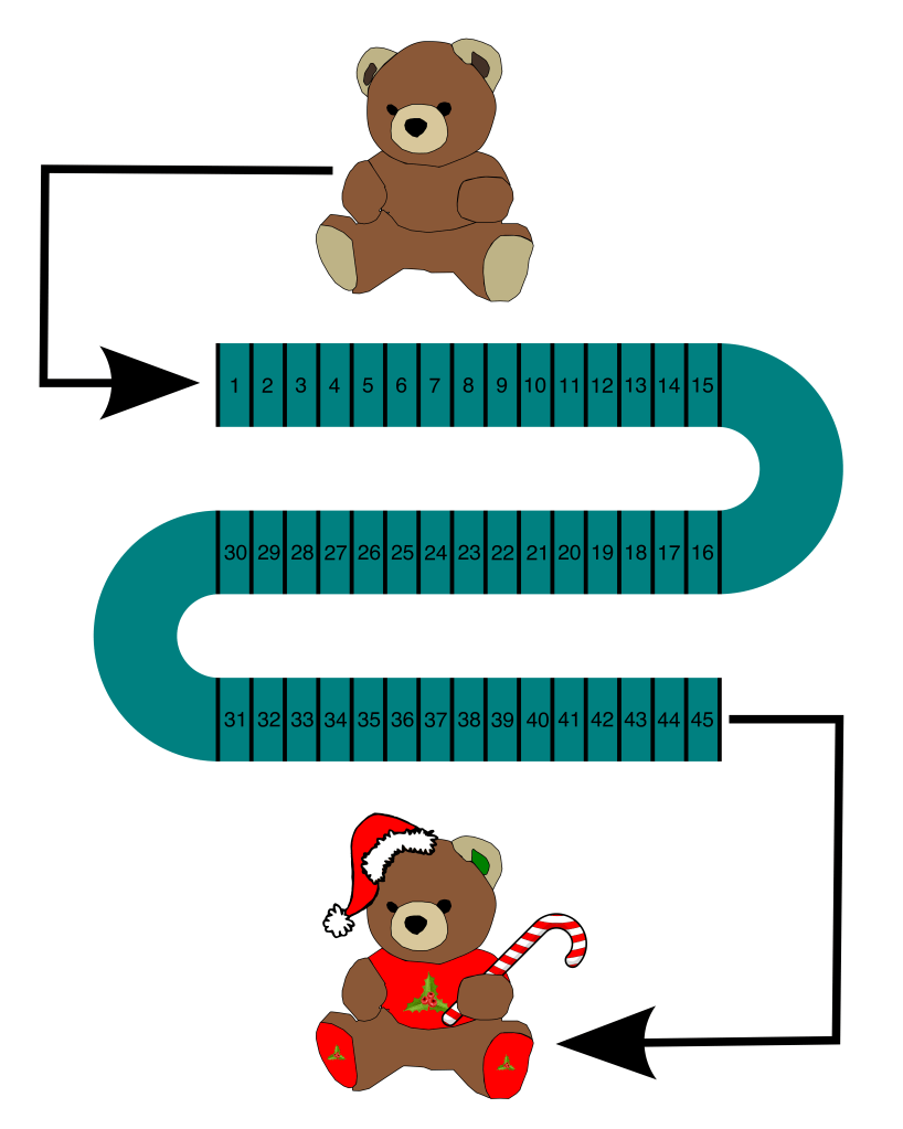
But enough of my yakking! My description of half-splitting is likely not enough to understand how it works in practice, so let’s look at an example. Let’s consider an automated assembly line which decorates teddy bears. An unfinished teddy bear enters the line and, at various stations along the way, is decorated and dressed:

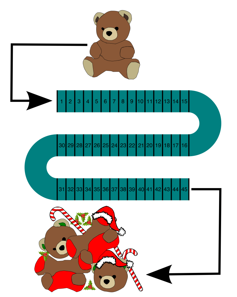
Today, something has gone terribly wrong: the unfinished bears go in one end, and out comes a pile of junk on the other!

Clearly, something is severely malfunctioning and destroying our teddy bears. But where is the problem? There are a lot of stations to check on the assembly line: 45 in all. We need the teddy bear assembly line up and running ASAP—after all, fake fur is money. To add to our difficulties, the assembly line is completely covered and therefore we can’t see what’s going on inside. There are access hatches above each station, but going through the line and checking all of them one-by-one is going to take a long time. Instead, we’ll use the half-splitting technique to speed up the process, find the cause, and get the line rolling again.

First off, we want to divide the assembly line into 2 equal parts. There are 45 stations, so the middle station is #23 (there are 22 stations on either side of #23). We open the hatch over station #23 and take a look:

At station #23, the teddy bears are fine. The assembly line flows from station #1 to station #45. By verifying the correct operation of station #23, we know the problem lies further downstream. Think about what we just did: in one fell swoop, we eliminated stations #1-23 as the cause of our bear tragedy. That’s a very efficient use of our time!

Now, we know that the problem lies somewhere within stations #24-45. So, let’s half-split again: the middle station between #24-45 is #35. Inspecting #35, we find good bears once again. Hooray again for our potent efforts: another 12 stations (#24-#35) were eliminated in a single action! We’re on a roll, so we’ll continue splitting and inspecting until we find the cause. This table shows our progress as we narrow in on the cause:

Iteration	Lower Bound	Upper Bound	# of Remaining Possibilities	Middle	Middle Status	Next Split
1	1	45	45	23	OK	→
2	24	45	22	35	OK	→
3	36	45	10	41	FAULT	←
4	36	40	5	38	FAULT	←
5	36	37	2	37	FAULT	←
6	36	36	1	36	OK

A summary of what we did: after our initial two splits, we knew the problem was between #36-45 (the lower and upper bounds listed for iteration #3). We examined the middle station (#41), and found a mangled pile of bear parts! Whenever you find a failure, you know that the problem must lie at that station or before, and therefore the next split you make will be backwards. So, that’s what we did in iteration #4: we split backwards and examined #38 (which also turned out to be a failing station). This leaves only 2 stations (#36 and #37), and we look at both of them because we want to verify the transition point from working to failed. Station #37 has a pile of things that used to be a teddy bear, while station #36 is fine. We’ve found a working station followed by a failing station, and that means we’ve found the culprit: station #37 must be the one wreaking havoc!

In any chained system, finding a working node immediately followed by a failing node is the jackpot. Half-splitting accelerates this process, and the table shows the very quick narrowing of the range in which the error was located: 1-45 → 24-45 → 36-45 → 36-40 → 36-37 → 37. As a consequence of this, the number of remaining possibilities dramatically drops by half after each iteration: 45 → 22 → 10 → 5 → 2 → 1. It only took us 6 steps to find the error, whereas if we had gone serially from the beginning until the error was discovered, it would have taken 37 steps!

To clarify the process, when there is a single “weak link in the chain,” the goal is to find the first failing node. In these type of systems, everything before that first failing node will work, and everything after it will not. Here’s a visual representation of how this works:

Half-splitting vs Serial Search

Half-splitting will quickly identify that first failing node in a chain. The larger your system, the bigger the payoff in terms of time saved. Let’s see how half-splitting and serial search measure up in systems of various sizes:

Chain Length	Total Inspections		Average Inspections		Advantage
	Serial	Half-splitting	Serial	Half-splitting
2	3	4	1.50	2.00	SERIAL
3	6	6	2.00	2.00	EVEN
4	10	10	2.50	2.50	EVEN
5	15	14	3.00	2.80	HALF-SPLITTING
6	21	18	3.50	3.00	HALF-SPLITTING
7	28	21	4.00	3.00	HALF-SPLITTING
8	36	26	4.50	3.25	HALF-SPLITTING
9	45	31	5.00	3.44	HALF-SPLITTING
10	55	36	5.50	3.60	HALF-SPLITTING
15	120	60	8.00	4.00	HALF-SPLITTING
20	210	90	10.50	4.50	HALF-SPLITTING
50	1,275	288	25.50	5.76	HALF-SPLITTING
100	5,050	674	50.50	6.74	HALF-SPLITTING
1,000	500,500	9,978	500.50	9.98	HALF-SPLITTING
10,000	50,005,000	133,618	5,000.50	13.36	HALF-SPLITTING

To create this table, I wrote a computer program to generate all the possible initial error positions for a chain of a given length (if you’re interested, the source code is included in the notes at the end). Before we get into that, let’s review what we know about chain-like systems. I use the term “chain-like” to mean any system where the output from the first node is fed into the second, the second into the third, and so on until the end. As noted in “Follow The Chain,” errors will typically propagate along a chained system in two different ways:

• The output at the end of the chain will be flawed in some way.
• There will be no output.

The predictable, one-way flow of these kinds of systems confers an advantage for troubleshooting: when you find an error, you know that it must have originated somewhere upstream!

In the table, you can see that the serial and half-splitting methods are evenly matched at the start. Serial search even wins the first round (systems with 2 elements), and then it’s a tie for 3-4. However, after the systems grow to 5 elements, half-splitting starts to pull away. At 15, half-splitting finds the cause twice as quickly. By the time we get to 1,000 nodes, half-splitting’s advantage is overwhelming: 50 times faster! Remember, these aren’t just numbers, they’re how much time it would take you to find the cause. Interested in working 50 times as long?

The Tipping Point: 5 Elements

To get a better understanding of how the two methods compare, let’s examine a chained system with 5 nodes. This is a good example to look at because it’s the point where half-splitting gains the advantage over serial search. Even though the average number of inspections are nearly the same (2.8 vs 3) for this number of elements, there are some important differences I want to point out. Let’s start by listing all the possibilities for the location of a single error in a system with 5 elements, and see how the error propagates down the chain for each:

Scenario #	Node 1	Node 2	Node 3	Node 4	Node 5	Failing Node
1	FAULT	FAULT	FAULT	FAULT	FAULT	1
2	OK	FAULT	FAULT	FAULT	FAULT	2
3	OK	OK	FAULT	FAULT	FAULT	3
4	OK	OK	OK	FAULT	FAULT	4
5	OK	OK	OK	OK	FAULT	5

For the serial search method, you’d start at node #1 and search up the chain until you find an error. For possibility #1, you can see that you’d find the error right away, with just a single inspection (because the error is at node #1). For possibility #2, it takes 2 inspections, 3 for possibility #3, 4 for possibility #4, and 5 for the last possibility. Using the half-splitting method on a system with 5 nodes, you always start at node #3 (the middle) and then move forwards or backwards, based on what you find. Here’s a table comparing the number of inspections taken by half-splitting and serial search for all of the possible error locations:

Fault Position in a 5-node Chain	Serial Inspections	Half-splitting Inspections
1	1	3
2	2	3
3	3	2
4	4	3
5	5	3
Total	15	14
Average	3	2.8
Median	3	3
Variance	2.5	0.2

Going over the statistics, you can see that the totals and averages are nearly the same, while the median is identical. What’s remarkably different is the variance, which is a statistical measurement of sprawl for a group of numbers: the more spread out they are, the higher the variance. It’s easy to see why the variance is higher for serial search: its range of inspections is 1-5, while the range for half-splitting is 2-3.

Let’s imagine a case where the inspection of each element in our 5-element system takes one hour to complete. That would mean the serial search method could take anywhere from 1 to 5 hours to complete. Half-splitting, in contrast, would never take more than 3 hours. That kind of predictability could be highly prized among your customers.

Based on the data I generated, my recommendation is to use serial search when the number of elements is 4 or less. Serial has other advantages at this level: it’s easier to execute and keep track of the process. However, if controlling the variance of repair times is a big concern for your particular situation, then only use serial search for systems with 2 elements (and half-splitting for all the rest).

The Math Behind Half-splitting

When using the half-splitting method, the approximate number of times you’ll need to divide your system and inspect an element is described by this formula:

log2n

Where n is the number of elements in your system. Logarithmic functions grow slowly (compared to linear functions), and are considered the standard when writing scalable algorithms in the world of computer science. You get a good sense of the power of logarithmic functions when you look at really large data sets. Consider how quickly half-splitting finds the error in a chained system of 1,000,000 components:

log2(1,000,000) = 19.93

Only about 20 steps: that’s efficient! Contrast this with the formula for the average number of steps required by the serial search method:

(n + 1) ÷ 2

Again, n is the number of components in your system. A downside for the troubleshooter is that this function grows linearly with the size of the chain. That means that a serial search for an error in a chain of one million components would take:

(1,000,000 + 1) ÷ 2 = 500,000.5

That’s right, on average about a half-million steps!

The Right Stuff

Half-splitting requires a system where you can inspect any single element and, based on its state, know where to look next. That’s why it’s especially suited for transformational or logistical chains: assembly lines, data networks, computer programs, pipelines, electrical circuits, etc. In our teddy bear example, we could examine a particular station on the assembly line and, based on the condition of the bear, know whether the problem was upstream or downstream.

In the field of computer science, the same technique speeds lookups in long lists of sorted information (in computer science, the method is known as “binary search”). Opening a sorted list and inspecting the middle entry, you call tell if the piece of data you’re seeking is forwards or backwards in the list. Again, the key is knowing where to look next based on any one element.

The Wrong Stuff

You can’t split every problem in half and get the efficiencies described here: as noted, the ability of a single element to tell you the direction of the problem is the key for half-splitting. If you were working on a broken car, you wouldn’t gain anything from saying: “Let me split this problem in half, I’m going to see if the failure is on the right-hand side of the car.” Inspecting a random windshield wiper or a spark plug on the right-hand side of a car won’t tell you in which direction the problem lies. A car, taken as a whole, is a collection of independent subsystems: in that sense, there’s really no “middle” to split! Some of the chain-like subsystems on a car (fuel, electrical, etc.) would benefit from half-splitting, but only after other strategies have identified them as candidates for further investigation.

Notes and Computer Code:

PlanetMath’s page on the binary search algorithm says the “average-case runtime complexity” is approximately:

log2n − 1

The context given for the PlanetMath wiki page is dictionary lookups, which is similar to the use of half-splitting when troubleshooting: each iteration halves the number of possibilities leading to big efficiencies as the size of the data set grows. However, the use isn’t exactly the same and I wanted to compare actual numbers. I needed a way to generate real data comparing both methods in the context of troubleshooting. The data I generated was very close to the “log2n − 1” approximation. However, I found half-splitting for the purposes of troubleshooting is closer to just log2n. It would be cool to have a formula that gave the exact answer! I’m not a mathematician, so I’m not sure if this is even possible. Any takers to figure it out?

For the half-splitting program I wrote, it took a while for me to figure out the correct algorithm to detect the position of the initial error. For my first few tries, my implementation took a lot more steps than what I considered to be the ideal. The breakthrough came when I noticed that, if the last and current “middles” chosen by the algorithm converged, the answer had been found. This insight replaced a tangled mess of “if” statements in my code. I also made the decision to record the unique number of times the program examined a particular chain element. This brought the number of inspections in line with what I had experienced doing the algorithm by hand on paper. I also think this better simulates what a person would experience: specifically, in real life, anytime you notice a “WORKING” element followed by an “ERROR,” you know you’ve found the failing node. With the “converging middles” solution, sometimes the computer will take an extra step that a human wouldn’t. You could probably code this intelligence into the program, but I liked the simplicity of the “converging middles” code and so I decided to leave it alone. If you have a better solution, feel free to post it!

Anyway, here’s the program I wrote (in ruby) to simulate and compare the serial and half-splitting methods of troubleshooting:

#serial_vs_half_splitting.rb
#Author: Jason Maxham, https://artoftroubleshooting.com/
#Purpose: to simulate and compare troubleshooting of "chain-like" systems
#(assembly lines, pipelines, networks, etc.) with both the serial and 
#half-splitting methods. May the best algorithm win!

def create_chain(chain_length, first_error_position)
  chain = []
  for chain_position in 1..chain_length
    if chain_position < first_error_position
      chain.push("WORKING")
    else
      chain.push("ERROR")
    end
  end
  return chain
end

def find_error_by_half_splitting(chain)
  #we need to set and keep track of these variables:
  lower_bound = 0
  upper_bound = chain.length - 1
  last_chain_middle = ''
  #keep track of the elements we've inspected to compare to the serial method
  inspections = {}

  #do the first split and inspection
  range_length = upper_bound - lower_bound
  chain_middle = (range_length.to_f / 2.to_f).ceil
  inspections[chain_middle] = 1

  while 1 do
    if (chain[chain_middle] == "WORKING")
      #error is forwards in the chain: split forwards, set the 
      #lower bound to the current middle element plus 1
      lower_bound = chain_middle + 1
    else
      #error is backwards in the chain: split backwards, set the 
      #upper bound to the current middle element minus 1
      upper_bound = chain_middle - 1
    end
    inspections[chain_middle] = 1

    #set the last_chain middle to the current one
    last_chain_middle = chain_middle
    #calculate new middle
    chain_middle = ((lower_bound + upper_bound).to_f / 2.to_f).ceil

    #It's all over when: the current and previous middles converge
    if (last_chain_middle == chain_middle)
      return inspections.length, last_chain_middle + 1
    end
  end
end

def find_error_serially(chain)
  inspections = 0
  first_error_position = 0
  chain.each_with_index do |element, index|
    inspections += 1
    if element == "ERROR"
      first_error_position = index + 1
      #stop, we've found it!
      break
    end
  end
  return inspections, first_error_position
end

def generate_chains(chain_length)
  #we'll keep track of the number of times that the serial and half-splitting 
  #methods find a different initial error. NOTE: this should never happen,
  #but it was useful when I was debugging!
  num_errors = 0

  #also keep track of the number of times we looked at an element in the chain. 
  #the point of this exercise was to see how much more efficient 
  #half-splitting is versus serially searching through the elements
  #of a real system when troubleshooting.
  total_serial_inspections = 0
  total_hs_inspections = 0

  #create chains, with the initial error in every possible position
  for initial_error_position in 1..chain_length
      chain = create_chain(chain_length, initial_error_position)
      (serial_inspections, serial_error_position) = find_error_serially(chain)
      (hs_inspections, hs_error_position) = find_error_by_half_splitting(chain)
      unless (serial_error_position == hs_error_position)
        num_errors += 1
      end 
      total_serial_inspections += serial_inspections
      total_hs_inspections += hs_inspections
  end
  return num_errors, total_serial_inspections, total_hs_inspections
end

def serial_vs_half_splitting
  total_errors = 0
  total_serial_inspections = 0
  total_hs_inspections = 0

  calculate_these = (2..20).to_a
  calculate_these.push(50,100,1000,10000)

  calculate_these.each { |chain_size|  
      (errors, s_inspections, hs_inspections) = generate_chains(chain_size)
      puts "#{chain_size}\t#{s_inspections}\t#{hs_inspections}\t#{(s_inspections.to_f / chain_size.to_f)}\t#{hs_inspections.to_f / chain_size.to_f}"
      total_errors += errors
      total_serial_inspections += s_inspections
      total_hs_inspections += hs_inspections
  }

  puts "SERIAL AND HALF-SPLITTING DIDN'T FIND THE SAME ANSWER: #{total_errors} TIMES"
  puts "SERIAL SEARCHING REQUIRED #{total_serial_inspections} INSPECTIONS OF CHAIN ELEMENTS"
  puts "HALF-SPLITTING REQUIRED #{total_hs_inspections} INSPECTIONS OF CHAIN ELEMENTS"
end
serial_vs_half_splitting

References:

• Header image: Mason Kimbarovsky, photographer. Retrieved from Unsplash, https://unsplash.com/photos/qEwJFHU3uOE.
• PlanetMath, Binary Search.