Interconnected systems can suffer from the presence of bottlenecks: individual components that limit the speed of the system as a whole. Limitations like these are an interesting concept because every system has a ceiling to its throughput. If you buy a printer that can churn out a maximum of 10 pages per minute, you probably wouldn’t think of it as having a bottleneck, even though there’s some component inside that ultimately restricts it to that particular speed. However, a throughput of 10 pages per minute would definitely be an annoyance for a printer that was advertised as capable of 30 pages per minute. When a machine is operating normally, its capacity, though finite, is simply part of your assumption for how it should function. However, when a machine’s capacity fails to meet expectations—now we’re dealing with a bottleneck!
My point isn’t that bottlenecks aren’t real, but they are qualitative and exist in relative terms: “It’s going too slow!” is the cry that is often heard. But, slow compared to what? When a system’s capacity is not enough to meet demand (compared to some ideal standard), then the cause of the limited throughput is called a bottleneck. Identifying the standard is important, because dealing with bottlenecks often blurs the line between troubleshooting and engineering. When a system is bottlenecked because of a malfunction, then this is clearly the domain of troubleshooting: the system had a certain throughput in the past, and the goal is to get it back there. However, when a system is employed in a new way, or when it’s asked to do more than it should, it may bump up against its design limitations. When that’s the source of the slowdown, overcoming those limits by expanding capacity or performance tuning isn’t technically troubleshooting.
I point this out because the people who say “Just make it go faster!” might not be aware of the distinction. From their perspective, all they know is that the system isn’t performing up to their expectations. It’s important for you, the troubleshooter, to keep this difference in mind: one path is about restoring functionality and the other is about making process improvements (or resetting expectations). If you’re responsible for a machine, you’ll likely be asked to investigate in either case, so we’ll discuss both. After explaining the situation to whomever is experiencing the problem, if you also include a clever way to improve capacity, you’ll look really sharp.
(image: Erich Ferdinand / CC BY 2.0)
The Weakest Link
Chained systems flowing along a single path will inevitably have nodes that complete their tasks at different speeds. There’s nothing wrong with this, it’s simply the nature of whatever the machine was designed to accomplish. If we’re talking about an oil refinery, the various sequential steps (fractional distillation, processing/cracking, treating/blending) are in different states of technological advancement. That one phase takes longer than another is a reflection of the nature of the work being performed and the amount of brainpower (i.e., innovation) that has been brought to bear on the problem. Processes that were once very slow might be comparatively quick now.
The problem with chaining processes together is that the overall throughput of the system will be limited by the rate of the slowest one. If a node in a chain can only handle one item at a time, it must wait for the next node to be clear before it can send its output down the line. If nodes have different completion times, some will finish early and sit idle. The strict definition of a bottleneck is “a narrowing”: the type of narrowing relevant to our discussion is a reduction in the rate of flow, observed when crossing between two nodes. I want you to see how this works, so let’s look at a simple 3-node assembly line system that paints Christmas Tree ornaments. Station A cleans the ornament, B paints it, and C dries the paint. A → B → C:
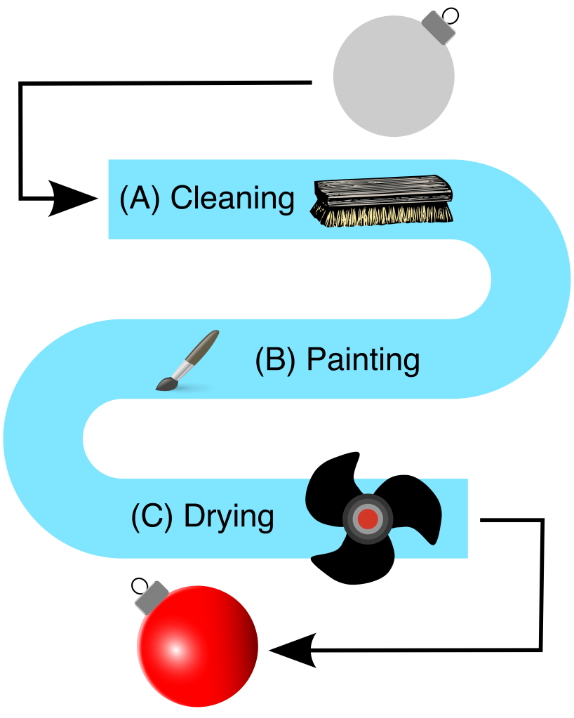
(image: © Jason Maxham)
The three steps have different completion times:
| Station | Work Performed | Completion Time (mins.) | Ornaments Per Hour | % Change In Speed |
| A | Cleaning | 5 | 12 | N/A |
| B | Painting | 10 | 6 | -50% |
| C | Drying | 20 | 3 | -50% |
Technically, we’ve got two bottlenecks here, right in a row! Going from A → B represents a 50% reduction in the rate of speed: 12 ornaments per hour to 6. Likewise for B → C, which goes from 6 to 3. Each of these transitions is a “narrowing” of the flow rate and therefore a bottleneck, but the slowest step (C) will ultimately control the overall rate of this system. Here’s a chart showing the progress of 4 ornaments (numbered 1-4) passing through the stations (A-C) of the painting assembly line:
| Elapsed Time | Ornament #1 | Ornament #2 | Ornament #3 | Ornament #4 |
| 00:00 | START | START | START | START |
| 00:05 | A | START | START | START |
| 00:10 | B | A | START | START |
| 00:15 | B | A | START | START |
| 00:20 | C | B | A | START |
| 00:25 | C | B | A | START |
| 00:30 | C | B | A | START |
| 00:35 | C | B | A | START |
| 00:40 | DONE | C | B | A |
| 00:45 | C | B | A | |
| 00:50 | C | B | A | |
| 00:55 | C | B | A | |
| 01:00 | DONE | C | B | |
| 01:05 | C | B | ||
| 01:10 | C | B | ||
| 01:15 | C | B | ||
| 01:20 | DONE | C | ||
| 01:25 | C | |||
| 01:30 | C | |||
| 01:35 | C | |||
| 01:40 | DONE | |||
| Time Summary | ||||
| Ornament #1 | Ornament #2 | Ornament #3 | Ornament #4 | |
| Waiting Time | 00:00 | 00:15 | 00:25 | 00:25 |
| Completion Time | 00:35 | 00:50 | 01:00 | 01:00 |
First off, notice that the first ornament passed through the line in 35 minutes. This is just the sum of the completion times for the individual stations (5 + 10 + 20 = 35). Then things slow down a bit: the second ornament passes through the line in 50 minutes. What gives? You can see from the table that Ornament #2 spent 15 minutes waiting for Ornament #1 to finish (idle moments are shown in red, time spent working in green). Because a station can only handle a single ornament at one time, when it’s occupied the ornament coming behind must wait. For example, at the 10 minute mark, Ornament #2 was done with cleaning at Station A; however, it had to wait another 5 minutes for Ornament #1 to vacate Station B so it could move on. Things slow down even further with Ornament #3, which takes 60 minutes to get through the line. At this point, the total completion time stabilizes: Ornament #4 also takes 60 minutes to finish. Ornaments #3 and #4 each spend 25 minutes waiting for subsequent stations to open up.
Once the system is fully loaded, an ornament gets done every 20 minutes: 00:40, 01:00, 01:20, and 01:40. This is what we were talking about when we said that a chained system’s rate will be limited by the slowest node (in this case that’s the drying station, C).
Not Every Increase Matters
Now that we’ve got a basis for comparison, let’s look at what happens when a problem occurs in the painting line. Let’s say that the cleaning and painting stations (A and B) both use compressed air from the same air compressor. Over time, the compressor has degraded and now it takes longer to recharge and maintain the desired pressure level. This result is an increase in the work time for Stations A and B of 5 minutes each:
| Station | Work Performed | Completion Time (mins.) | Ornaments Per Hour | % Change In Speed |
| A | Cleaning | 10 | 6 | N/A |
| B | Painting | 15 | 4 | -33% |
| C | Drying | 20 | 3 | -25% |
We still have bottlenecks from A → B (-33%) and B → C (-25%), but they’re not as large, percentage-wise, as before. What remains the same is that Station C is still the slowest to complete its work at 20 minutes per ornament.
With the line slower, let’s see what happens when we send through four more ornaments (numbered 5-8):
| Elapsed Time | Ornament #5 | Ornament #6 | Ornament #7 | Ornament #8 |
| 00:00 | START | START | START | START |
| 00:05 | A | START | START | START |
| 00:10 | A | START | START | START |
| 00:15 | B | A | START | START |
| 00:20 | B | A | START | START |
| 00:25 | B | A | START | START |
| 00:30 | C | B | A | START |
| 00:35 | C | B | A | START |
| 00:40 | C | B | A | START |
| 00:45 | C | B | A | START |
| 00:50 | DONE | C | B | A |
| 00:55 | C | B | A | |
| 01:00 | C | B | A | |
| 01:05 | C | B | A | |
| 01:10 | DONE | C | B | |
| 01:15 | C | B | ||
| 01:20 | C | B | ||
| 01:25 | C | B | ||
| 01:30 | DONE | C | ||
| 01:35 | C | |||
| 01:40 | C | |||
| 01:45 | C | |||
| 01:50 | DONE | |||
| Time Summary | ||||
| Ornament #5 | Ornament #6 | Ornament #7 | Ornament #8 | |
| Waiting Time | 00:00 | 00:10 | 00:15 | 00:15 |
| Completion Time | 00:45 | 00:55 | 01:00 | 01:00 |
Looking at the numbers, some amazing and very counter-intuitive things have happened. First, idle times while in the queue have actually decreased! Ornament #6 waited 5 minutes less (versus Ornament #2 in our previous test run), while Ornaments #7 and #8 waited 10 minutes less each (versus #3 and #4). As far as time in the queue is concerned, Ornaments #7 and #8 took one hour to make it through the line, the same as before the compressor was having problems. Perhaps most astonishing is that the throughput of the system was exactly the same: once the system was loaded, an ornament rolled off the line every 20 minutes at 00:50, 01:10, 01:30, and 01:50!
Once again, we observe that the slowest station controls the pace of a chained system. We’ve also learned something new in this run: the limiting node can mask problems elsewhere. Because the total throughput remained the same, you might not have noticed the compressor problem until it was too late. Most importantly, if you’re troubleshooting a “it’s too slow” kind of problem in an interconnected system, you must focus on the narrowest bottleneck (i.e., the slowest station) for your efforts to have any effect.
Show Me The…Data!
How do we find that narrowest bottleneck so we know where to direct our efforts? The best case scenario to rapidly pinpoint the location of a bottleneck is operational data. If you had monitors recording the flow rate at each of the stations in the ornament assembly line, you could easily see a decrease in speed either numerically or graphically. However, that’s a level of preparation I rarely see, except for those organizations that have been badly burned by bottlenecks in the past (like mine!). Only at the very end of my tenure as a CTO could I lay claim to such a level of preparedness (by then I was a data fanatic), but even so we didn’t monitor everything. To find a bottleneck in a mass-produced, off-the-shelf item, it might be hard to add the type of probes necessary for this level of awareness.
Slow Your Roll, Even More
Let’s say you have a hunch that a particular link in a chain is the narrowest bottleneck. We know that the throughput of a chained system is controlled by the slowest node, so an easy way to vet a suspect is to slow it down even further! If the rate of output decreases further, you’ve found the limiting bottleneck. This is a great technique for digital systems, where flow rates can easily be adjusted with a line in a configuration file or some code added to a computer program.
In our ornament assembly line, Station C was the slowest and therefore controlled the pace of throughput. Therefore, if you slowed Station C down even further, the immediate result would be to decrease the rate that ornaments rolled off the line. Busted, Station C!
One important caveat for this technique is to choose the smallest possible increment when adding additional sloth to the suspected node. Remember, in a single-track system any node can become the controlling bottleneck. If you tip the scales with too heavy a hand, all you’ll learn is that you can make new bottlenecks. I think we knew that already!
Get Out That Stopwatch
Another way to determine the location of a bottleneck is to send a tracking probe down the chain and time its progress. In our painting assembly line, that would mean putting an ornament in the queue and taking note of when it enters and exits each of the stations. Digital systems will have these tools available in software: a programmer can add code to note the time spent in various functions, making database calls, etc. Analog or digital, having precise data of how time is spent in the system is invaluable. That’s because there’s another possibility we haven’t discussed: two or more identical “narrowest” bottlenecks! In our painting assembly line, if all three stations (A, B, and C) took 20 minutes to complete their work, you’d need to speed up all of them to achieve a faster system.
Half-splitting To Find The Bottleneck
Ideally, you’d have timing data on every node in a system so that there would be no mystery as to the location of the bottleneck. However, there will be times when collecting such data will come at too high a price: either the probe will be hard to track as it moves through the system, access may be limited, or it just requires a lot of manual labor.
What if you could only collect one data point at a time? What would give you the most bang for your buck? Ding, ding, ding! You’re right: we can half-split our way to finding the bottleneck and save a lot of effort. We reviewed half-splitting in detail in “Clear Up To Here”: remember the teddy bear assembly line? Let’s use that example again, but this time in the context of a slowdown. Imagine that a bear normally completes the trip from “naked” to “Christmas fabulous,” passing through all 45 assembly line stations, in about 15 minutes (an average of ~20 seconds per station). However, today it’s taking 60 minutes for a bear to emerge from the line. I smell a bottleneck.
We’ll start by dividing the system in two and then collecting data at the mid-point (again, Station #23). We’ll mark a special test bear with a big red “Test” across its face to distinguish it from the rest, and then we’ll send it on down the line. Opening up the access hatch over Station #23, we’ll wait for our test bear to pass the mid-point, noting the time when it crosses (in addition to the starting and ending times):
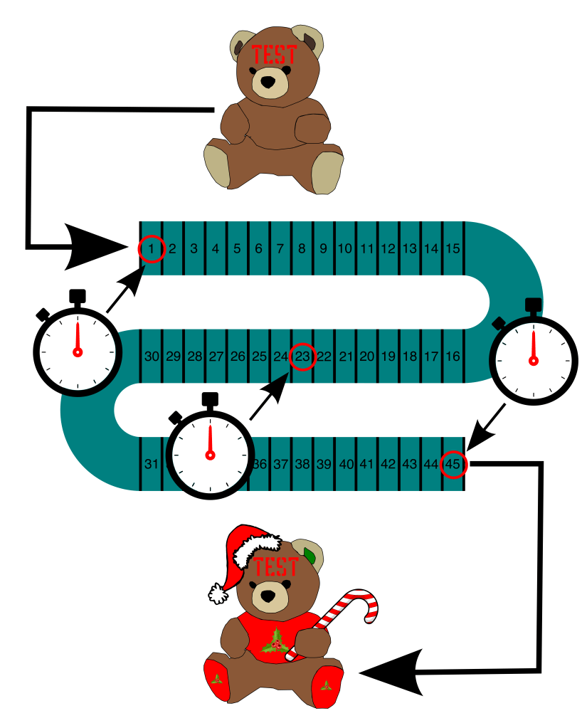
(image: © Jason Maxham)
These are the timings we get:
| Station Location | Time Elapsed |
| Start | 00:00 |
| #23 | 00:48 |
| End | 01:00 |
You can see that it took 48 minutes for the test bear to reach Station #23. That means the time it takes to go through the first half of the line (48 minutes) is 4 times longer than the second half (12 minutes)! This is a very strong indication that the bottleneck is located between Stations #1-23. Just like before, we can continue half-splitting until we’ve narrowed it down further. If that was necessary, the next step would be to send another test bear down the line and take a reading at Station #12. But, maybe the first split is good enough to jump-start an investigation. Remember, half-splitting is a very efficient way of eliminating possibilities. Let’s say, based on other evidence, you had a solid list of three suspects: Stations #12, #30, and #40. The timings from our initial split indicate the bottleneck is in the first half of the assembly line, thereby eliminating #30 and #40. At that point, I wouldn’t split further, and instead head right to Station #12.
Make It Go Faster
I’ve spilled a lot of ink talking about how bottlenecks work and how to find them. Of course, there’s that last step: making the system as a whole go faster. If you find that the narrowest of narrows is the result of a malfunction, then it’s just a matter of making the correct repair. However, another possibility is that the system is now being asked to do something that’s beyond its capability or capacity. Or, the system can be performing exactly as intended: some machines are designed to slow down under certain types of workloads. Rectifying these scenarios can be much harder. Basically, your options for the bottlenecked node are:
- Make it go faster.
- Make it do less.
- Stockpile.
- Parallelize.
The first one is self-explanatory: zoom zoom! As for number 2, “doing less” can mean any number of optimizations, but the basic idea is that scrutiny will often reveal unnecessary work being done by the bottlenecked node. Stockpiling means running the bottlenecked system more (perhaps even 24/7/365) and storing its output to smooth out swings in demand. Unfortunately, this entails inventory and storage costs, and doesn’t help systems that must do “on-demand” work. Parallelizing is where you deploy multiple systems to simultaneously handle the workload of the bottlenecked node. Like widening a one-lane road, this means work can be performed in parallel along multiple pathways. In our painting assembly line, drying was our bottleneck. To double the speed of that task, we could add a second drying station:
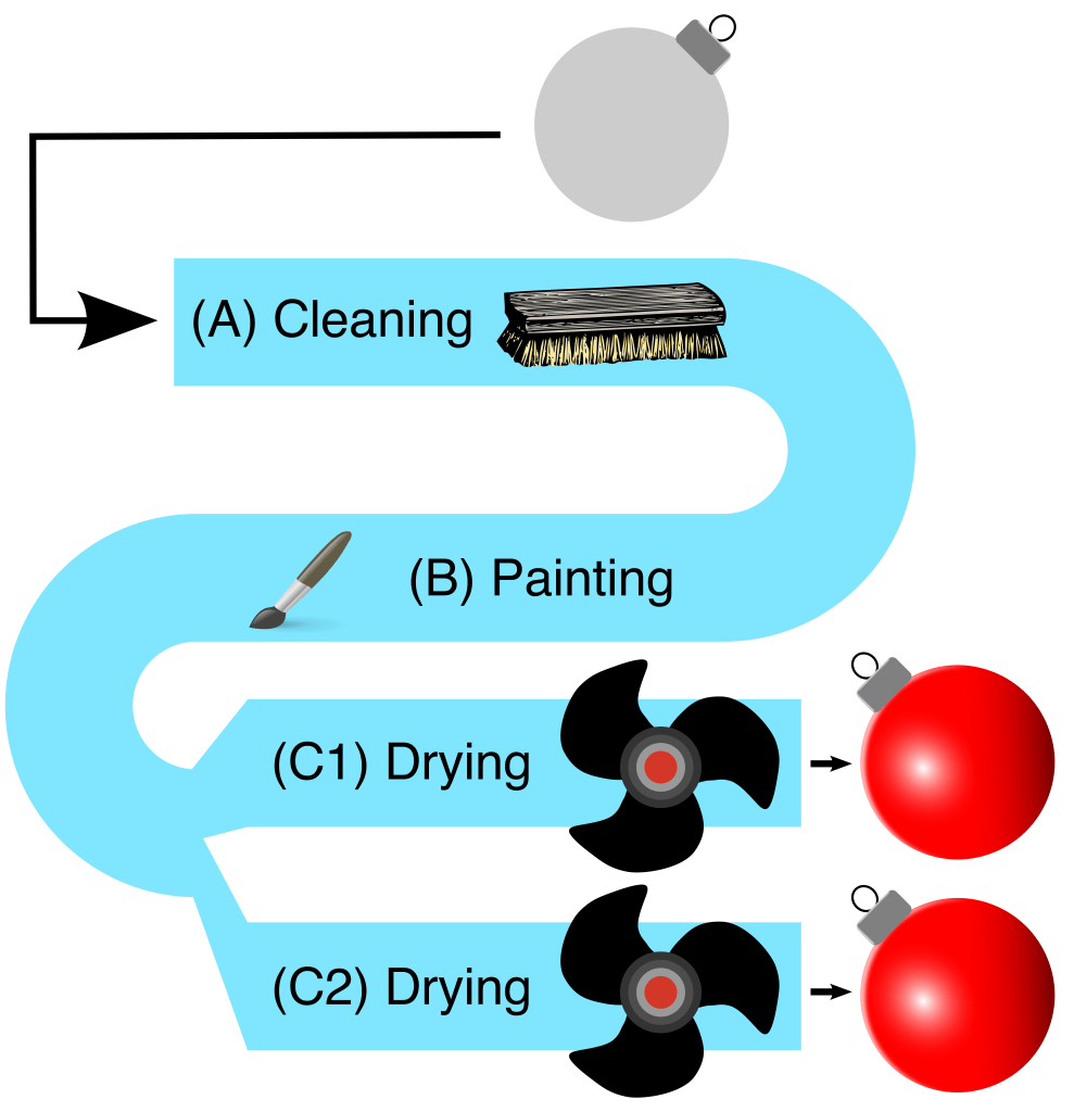
(image: © Jason Maxham)
This is the kind of thing that’s very easy to mock up in PowerPoint, but much harder to actually pull off in a working factory. Removing bottlenecks with parallelization to meet growing demand can be a golden ticket or your worst nightmare. When it comes to scaling, some companies make it, and some don’t. Finally, remember that optimizing bottlenecks is like a game of Whac-A-Mole: speeding up one part of a system will make some other part the slowest. Once you’ve dispatched a particular bottleneck, another one will appear! With Whac-A-Mole, you stop when the game is over. With bottlenecks, you stop when your company is wildly profitable.
Things Need To Be Just Right
Then Goldilocks went upstairs into the bedchamber in which the three Bears slept. And first she lay down upon the bed of the Great, Huge Bear; but that was too high at the head for her. And next she lay down upon the bed of the Middle Bear; and that was too high at the foot for her. And then she lay down upon the bed of the Little, Small, Wee Bear; and that was neither too high at the head, nor at the foot, but just right. So she covered herself up comfortably, and lay there till she fell fast asleep.
The Annotated Classic Fairy Tales 1
After you’ve fixed your fair share of bottlenecks, you might achieve that rare honor of making something go too fast. Your record-setting innovation may flood downstream nodes with an excessive amount of work. That’s happened to me: I’ve released bottlenecks that were actually protecting the system with their sluggish ways. When that happens, you’ll need to install governors to return the flow rate back to a level that can be sustained. Tuning involves fixing things that are too slow, as well as too fast. The best of luck as you work to get things just right.
References:
- Header image: Road construction delays traffic on West Side Highway, at 79th Street, New York City, during rush hour. World Telegram photo by Al Ravenna. New York, 1951. [Photograph] Retrieved from the Library of Congress, https://www.loc.gov/item/94505641/.
- 1 Maria Tatar, The Annotated Classic Fairy Tales, (New York: W. W. Norton & Company, 2002), pg. 249.
